Simulated Conditional Formatting part 2

Thanks again to Srinivas Dandamudi for posting the previous example on Simulating Conditional Formatting! 🙂

It works great as a brute force method, however we would need to have a total of 3 objects per cell (100 cells = 300 objects). In addition, we would have to replicate the the behaviour of each cell and carefully place them which would take a long time even for 10 cells.

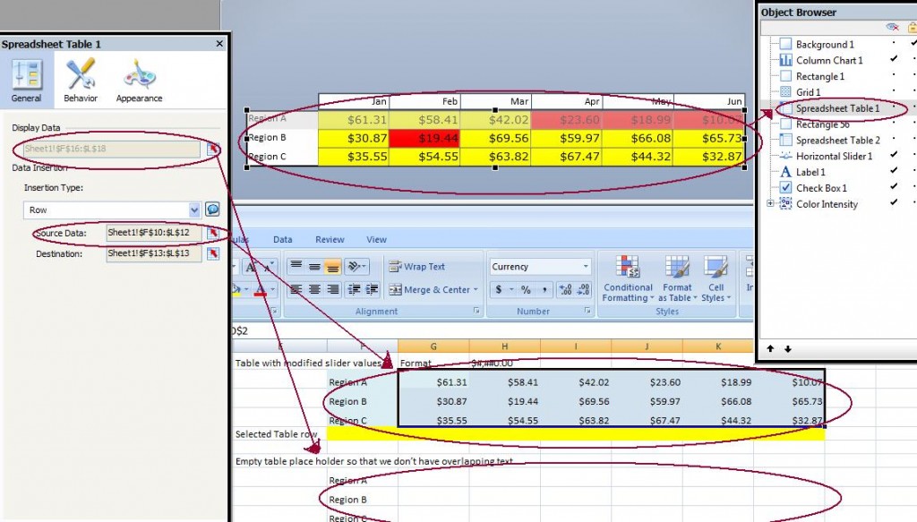
Instead of using a seperate rectangle for each cell, we can use a grid and enable alerts on the grid. To simulate the table selector, you can just overlay a spreadsheet table object on top of the grid. The key here is to choose an empty display area for the table so that we don’t have overlapping text.

Here are the steps to accomplish the trick

Step 1:
Insert a grid object.

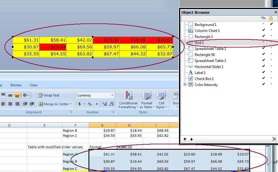
Step 2:
Setup the grid alerts based on the value of each cell.

Step 3:
Overlay the spreadsheet on top of the grid if you want to be able to select the rows like the example on part 1.
Make sure that the display data is pointing to cells that are empty so that we dont have overlapping text

The source code can be found here [download id=”2″]

Note that I’ve used Srinivas’ previous source code and removed a bunch of stuff both in the Excel and Xcelsius file to make things simpler to understand.